After spending quite a bit of time making my Matlab figures look the way I like, I wanted to record it both for my own reference and perhaps to aid others. The following are my notes.
To follow along, one could use the following values.
xDat=[0:100];
yDat=xDat;
R = sqrt(xDat.^2 + yDat.^2) + eps;
zDat = sin(R)./R;
xSize=2.02;
ySize=3.25; %related by the golden ratio
[X,Y] = meshgrid(-8:.5:8);
R = sqrt(X.^2 + Y.^2) + eps;
Z = sin(R)./R;
Essential formatting: one plot figure
For many graphs, there is a figure that contains one plot, with an x and y axis. The basic formatting for this is as follows. For all of the exampls xDat and yDat are the data series x and y values respectively.
- Start with giving a figure number:
figure(11) - turn
hold on;so that nothing is updated until all the commands are given. - give the plot:
plot(xDat,yDat),semilogy(xDat,yDat), or, if multiple data sets in a loglog plot,loglog(xDat1,yDat1,'k+',xDat2,yDat2,'ko'). - set the x and y axis labels:
ylabel('a_s (a_0)'); xlabel('\lambda'); - set the renderer and background color:
set(gcf, 'renderer', 'painters'); set(gcf, 'color', 'white'); - I prefer boxes around my figures:
box on; - Turn
hold off;
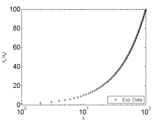
An example thus looks like, with the addition of modifying the axis boundries, the font size, and adding a legend.
figure(3)
plot(xDat,yDat, 'k+')
ylabel('a_s (a_0)');
xlabel('\lambda');
set(gcf, 'renderer', 'painters');
set(gcf, 'color', 'white'); % sets the color to white
set(gca,'XScale','log');
xlim([0 100]);
ylim([0 100]); %could also use axis([0 100 0 100]);
set(gca,'FontSize',18);
l1=legend('Exp. Data','Location','SouthEast');
set(l1,'FontSize',12);
hold off;
This results in a figure that looks ready to publish, perhaps with a few more tweaks to the font sizes:

Saving to a file can easily be accomplished too. Just add a
print(gcf, '-dpdf', 'fileName.pdf');
for example to save a pdf version of the file. Or, if a png, jpeg, or tiff, format is wanted, use '-dpng', '-djpeg', or '-dtiff' respectively in place of '-dpdf'.
Printing to paper
Getting the figure to be a specific size when saved or printed, however, takes a couple extra steps. One needs to specify the paper size and the position of the figure on the piece of paper. An example follows:
set(gcf, 'PaperUnits', 'inches');
set(gcf, 'PaperPositionMode', 'manual');
set(gcf, 'PaperSize', [xSize ySize]);
set(gcf, 'PaperPosition', [0 0 xSize ySize]);
where xSize and ySize are numbers set in inches.
Further control is possible by defining the axis poisition and size, as follows:
ax1=axes('position',[ .2,.1,.8,.8]);
For the position property, the order is [left bottom width height] in which each is defined as a fraction of the total figure size (0.0-1.0). Saving the figure at this point will give a figure that could be printed and will be the size as defined by the values given to xSize and ySize.
3D surface plots
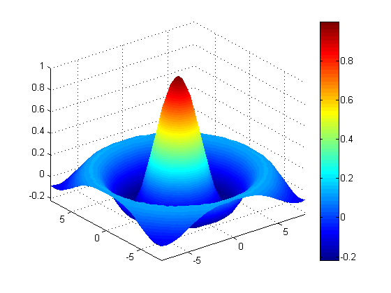
I prefer the following lighting, shading and styles for my surface plots.
surf(X,Y,Z,'EdgeColor','none');
axis tight;
shading interp;
lighting phong;
set(gcf, 'renderer', 'painters');
set(gcf, 'color', 'white');
colorbar
This results in a ready-to-go surface plot:

Multiple plots in one figure
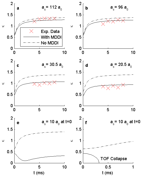
For more complicated figures with multiple plots, a new addition is needed. At this point, one can either use subplot which employs Matlab's native multiple plot in one figure layout. I, however, have found that very unsatisfactory for giving good plots. Instead, I recommend using an invisible axis as the main axis, and defining all the rest of the axis relative to that. Here's how that would be done with 6 axis all in one figure (note, the data is not supplied).
figure(85);
%hold on;
axbkgd=axes('Position',[0 0 1 1],'Visible', 'off');
axis([0 1 0 1]);
%formatting figure
set(gcf, 'renderer', 'painters');
set(gcf, 'color', 'white'); % sets the color to white

set(gcf, 'PaperUnits', 'inches');
xSize = 4; %inches wide for total page
ySize = 5; %inches high for total page
axisLeft = .1;
axisRight = .58;
axisTop = .73;
axisMiddle = 0.41;
axisBottom = .09;
axisXSize = .35;
axisYSize = .25;
axisInsetSize = .1;
InsetLeft = .30;
InsetBottom = .12;
set(gcf, 'PaperPositionMode', 'manual');
set(gcf, 'PaperSize', [xSize ySize]);
set(gcf, 'PaperPosition', [0 0 xSize ySize]);
fntsize=8;

%%%%FIGURE UPPER LEFT
ax1=axes('position',[axisLeft,axisTop,axisXSize,axisYSize]);
set(ax1,'FontSize',fntsize);
h1=plot(fig4a_t,fig4a_aspect,'rx', t4a,asp4a, 'k-',t04a,asp04a, 'k-.');
ylabel('\kappa');
axis([0 10 0 2]);
text(.5,1.8, 'a','FontSize',fntsize, 'FontWeight','bold');
text(5.5,1.8, 'a_s= 112 a_0','FontSize',fntsize);
l1=legend('Exp. Data','With MDDI', 'No MDDI','Location','SouthEast');
set(l1,'FontSize',fntsize);
box off

%%%%FIGURE UPPER RIGHT
ax2=axes('position',[axisRight,axisTop,axisXSize,axisYSize]);
set(ax2,'FontSize',fntsize);
h2=plot(fig4b_t,fig4b_aspect,'rx', t4b,asp4b, 'k-',t04b,asp04b, 'k-.');
ylabel('\kappa');
axis([0 10 0 2]);
text(.5,1.8, 'b','FontSize',fntsize, 'FontWeight','bold');
text(5.5,1.8, 'a_s= 96 a_0','FontSize',fntsize);
box off

%%%%FIGURE MIDDLE LEFT
ax3=axes('position',[axisLeft,axisMiddle,axisXSize,axisYSize]);
set(ax3,'FontSize',fntsize);
h3=plot(fig4c_t,fig4c_aspect,'rx', t4c,asp4c, 'k-',t04c,asp04c, 'k-.');
ylabel('\kappa');
axis([0 10 0 2]);
text(.5,1.8, 'c','FontSize',fntsize, 'FontWeight','bold');
text(5.5,1.8, 'a_s= 30.5 a_0','FontSize',fntsize);
box off

%%%%FIGURE MIDDLE RIGHT
ax4=axes('position',[axisRight,axisMiddle,axisXSize,axisYSize]);
set(ax4,'FontSize',fntsize);
h4=plot(fig4d_t,fig4d_aspect,'rx', t4d,asp4d, 'k-',t04d,asp04d, 'k-.');
ylabel('\kappa');
axis([0 10 0 2]);
text(.5,1.8, 'd','FontSize',fntsize, 'FontWeight','bold');
text(5.5,1.8, 'a_s= 20.5 a_0','FontSize',fntsize);
box off
set([h1,h2,h3,h4], 'MarkerSize',10)

%%%%FIGURE LOWER LEFT
ax5=axes('position',[axisLeft,axisBottom,axisXSize,axisYSize]);
set(ax5,'FontSize',fntsize);
plot(tWithMDDI, Asp, 'k-', tNoMDDI,Asp0,'k-.');
xlabel('t (ms)');
ylabel('\kappa');
xlim([0 10]);
ylim([0 2]);
text(.5,1.8, 'e','FontSize',fntsize, 'FontWeight','bold');
text(5.5,1.8, 'a_s= 10 a_0 at t=0','FontSize',fntsize);
box off;
set(ax5,'FontSize',fntsize);

%%%%FIGURE LOWER RIGHT
ax6=axes('position',[axisRight,axisBottom,axisXSize,axisYSize]);
set(ax6,'FontSize',fntsize);
plot(tWithMDDICollapse, AspCollapse, 'k-', tNoMDDICollapse,Asp0Collapse,'k-.');
xlabel('t (ms)');
ylabel('\kappa');
xlim([0 1]);
ylim([0 2]);
set(ax6,'FontSize',fntsize);
text(.35,.2, 'TOF Collapse','FontSize',fntsize);
text(.05,1.8, 'f','FontSize',fntsize, 'FontWeight','bold');
text(.55,1.8, 'a_s= 10 a_0 at t=0','FontSize',fntsize);
box off;
hold off;
The result, printed used '-dpng', looks like
